As far as literature searches go in the direction of cataloguing finite difference methods explicitly, there appears to be no descriptive representation of reaction–diffusion equations in their full three spatial dimensions. It is therefore our task (albeit tedious) to assemble the matrices and vectors for the model.
We extend the two-dimensional operator formulation to the
three-dimensional case by introducing an additional spatial index

with step size
.
The flux operators
are augmented by
the
-direction term
, so that the discrete diffusion operator
acting on the substrate
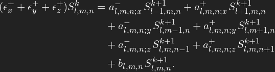
is given by the 3D seven-point stencil.
3D Stencil Formulation
(1) ![Rendered by QuickLaTeX.com \[ \begin{aligned} (\epsilon^{+}_x + \epsilon^{+}_y + \epsilon^{+}_z) S^k_{l,m,n} &= a^{-}_{l,m,n;x}\, S^{k+1}_{l-1,m,n} + a^{+}_{l,m,n;x}\, S^{k+1}_{l+1,m,n} \\ &\quad + a^{-}_{l,m,n;y}\, S^{k+1}_{l,m-1,n} + a^{+}_{l,m,n;y}\, S^{k+1}_{l,m+1,n} \\ &\quad + a^{-}_{l,m,n;z}\, S^{k+1}_{l,m,n-1} + a^{+}_{l,m,n;z}\, S^{k+1}_{l,m,n+1} \\ &\quad + b_{l,m,n}\, S^{k+1}_{l,m,n}. \end{aligned} \]](https://proteus-analytics.com/wp-content/ql-cache/quicklatex.com-06455bf9901879e277be8598f0c06783_l3.png)
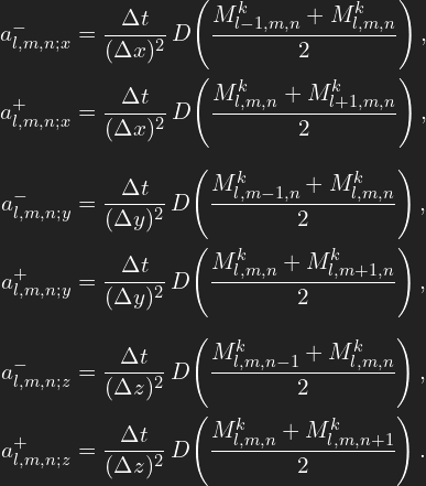
Coefficient Definitions
![Rendered by QuickLaTeX.com \[ \begin{aligned} a^{-}_{l,m,n;x} &= \frac{\Delta t}{(\Delta x)^2}\, D\!\left(\frac{M^k_{l-1,m,n} + M^k_{l,m,n}}{2}\right),\\ a^{+}_{l,m,n;x} &= \frac{\Delta t}{(\Delta x)^2}\, D\!\left(\frac{M^k_{l,m,n} + M^k_{l+1,m,n}}{2}\right),\\[6pt] a^{-}_{l,m,n;y} &= \frac{\Delta t}{(\Delta y)^2}\, D\!\left(\frac{M^k_{l,m-1,n} + M^k_{l,m,n}}{2}\right),\\ a^{+}_{l,m,n;y} &= \frac{\Delta t}{(\Delta y)^2}\, D\!\left(\frac{M^k_{l,m,n} + M^k_{l,m+1,n}}{2}\right),\\[6pt] a^{-}_{l,m,n;z} &= \frac{\Delta t}{(\Delta z)^2}\, D\!\left(\frac{M^k_{l,m,n-1} + M^k_{l,m,n}}{2}\right),\\ a^{+}_{l,m,n;z} &= \frac{\Delta t}{(\Delta z)^2}\, D\!\left(\frac{M^k_{l,m,n} + M^k_{l,m,n+1}}{2}\right). \end{aligned} \]](https://proteus-analytics.com/wp-content/ql-cache/quicklatex.com-63c66fabac8678e9e7293e8bf40fad9a_l3.png)
(2) ![]()
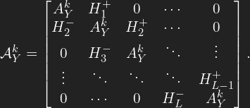
3D Block-Matrix Assembly
(3) ![Rendered by QuickLaTeX.com \[ \mathcal{A}^k_Y = \begin{bmatrix} A^k_Y & H^{+}_1 & 0 & \cdots & 0 \\ H^{-}_2 & A^k_Y & H^{+}_2 & \cdots & 0 \\ 0 & H^{-}_3 & A^k_Y & \ddots & \vdots \\ \vdots & \ddots & \ddots & \ddots & H^{+}_{L-1} \\ 0 & \cdots & 0 & H^{-}_L & A^k_Y \end{bmatrix}. \]](https://proteus-analytics.com/wp-content/ql-cache/quicklatex.com-444320bb1ea7c8e14ce15b9a0f50e092_l3.png)
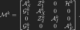
Global Coupled System
(4) ![Rendered by QuickLaTeX.com \[ \mathcal{M}^k = \begin{bmatrix} \mathcal{A}^k_S & \mathcal{Z}^k_1 & 0 & \mathcal{H}^k \\ \mathcal{G}^k_1 & \mathcal{A}^k_X & 0 & 0 \\ 0 & \mathcal{Z}^k_2 & \mathcal{A}^k_I & 0 \\ \mathcal{G}^k_2 & 0 & 0 & \mathcal{A}^k_E \end{bmatrix}. \]](https://proteus-analytics.com/wp-content/ql-cache/quicklatex.com-70d4274e1d095206ae683fdc82426b7d_l3.png)
Kronecker Representation
(5) ![]()